The Physics

Gravitational Acceleration

Every body in the system attracts every other body according to Newton’s Law of Universal Gravitation. For body $j$ , the net acceleration due to all other bodies $k$ is:

$\vec{a}_j = \sum_{k \neq j} \frac{G \, m_k}{r_{jk}^2} \, \hat{r}_{jk}$

where $r_{jk} = \lvert\vec{r}_k - \vec{r}_j\rvert$ is the distance between the two bodies and $\hat{r}_{jk}$ is the unit vector pointing from $j$ toward $k$ .

Why Initial Velocity Matters

Gravity alone will pull every body straight toward every other body. What prevents them from colliding is their initial velocity — the sideways motion that turns a free-fall into a curved orbit. This is the same reason the Moon doesn’t crash into the Earth: it’s falling toward us constantly, but it’s also moving sideways fast enough that it keeps missing.

When you call add_body(), the vx, vy, vz parameters set this initial velocity. The balance between speed and distance determines the shape of the orbit. At a given distance $r$ from a central mass $M$ , the circular orbit velocity is:

$v_{\text{circ}} = \sqrt{\frac{G \, M}{r}}$

If the body’s speed exactly matches this, it traces a perfect circle. Faster and the orbit stretches into an ellipse (or escapes entirely if $v \geq v_{\text{circ}} \sqrt{2}$ ). Slower and the orbit drops into a tighter ellipse that dips closer to the central body. With zero velocity, the body falls straight in — no orbit at all.

Gravitational Softening

When two bodies pass very close, $r \to 0$ and the acceleration diverges toward infinity. This is a well-known numerical problem in N-body codes. orbitr offers an optional softening length $\varepsilon$ that regularizes the potential:

$r_{\text{soft}} = \sqrt{r^2 + \varepsilon^2}$

With softening enabled, close encounters produce large but finite forces instead of blowing up to NaN. Set softening = 0 (the default) for exact Newtonian gravity, or try something like softening = 1e4 (10 km) for dense systems.

Numerical Integration Methods

simulate_system() offers three methods for stepping the system forward through time. All operate in 3D Cartesian coordinates.

1. Velocity Verlet (default, `method = "verlet"`)

A second-order symplectic integrator. It conserves energy over long timescales, making it the gold standard for orbital mechanics. Orbits stay closed and stable indefinitely.

$\vec{x}_{t+\Delta t} = \vec{x}_t + \vec{v}_t \, \Delta t + \tfrac{1}{2} \vec{a}_t \, \Delta t^2$

$\vec{v}_{t+\Delta t} = \vec{v}_t + \tfrac{1}{2} \left( \vec{a}_t + \vec{a}_{t+\Delta t} \right) \Delta t$

The position is advanced first, then the acceleration is recalculated at the new position, and finally the velocity is updated using the average of the old and new accelerations. This requires two acceleration evaluations per step (the main cost), but the payoff in stability is enormous.

2. Euler-Cromer (`method = "euler_cromer"`)

A first-order symplectic method. It updates velocity first, then uses the new velocity to update position. This small reordering prevents the systematic energy drift that plagues standard Euler:

$\vec{v}_{t+\Delta t} = \vec{v}_t + \vec{a}_t \, \Delta t$

$\vec{x}_{t+\Delta t} = \vec{x}_t + \vec{v}_{t+\Delta t} \, \Delta t$

Faster than Verlet (one acceleration evaluation per step) but less accurate. Good for quick previews.

3. Standard Euler (`method = "euler"`)

The classical textbook method. Position and velocity are both updated using values from the current time step:

$\vec{x}_{t+\Delta t} = \vec{x}_t + \vec{v}_t \, \Delta t$

$\vec{v}_{t+\Delta t} = \vec{v}_t + \vec{a}_t \, \Delta t$

This artificially pumps energy into the system, causing orbits to spiral outward over time. Included primarily for educational comparison — use Verlet for real work.

Comparing the Three Methods

library(orbitr)
library(dplyr)
#> 
#> Attaching package: 'dplyr'
#> The following objects are masked from 'package:stats':
#> 
#>     filter, lag
#> The following objects are masked from 'package:base':
#> 
#>     intersect, setdiff, setequal, union

system <- create_system() |>
  add_body("Star", mass = 1e30) |>
  add_body("Planet", mass = 1e24, x = 1e11, vy = 30000)

verlet <- simulate_system(system, time_step = seconds_per_hour, duration = seconds_per_year, method = "verlet") |>
  mutate(method = "Velocity Verlet")

euler_cromer <- simulate_system(system, time_step = seconds_per_hour, duration = seconds_per_year, method = "euler_cromer") |>
  mutate(method = "Euler-Cromer")

euler <- simulate_system(system, time_step = seconds_per_hour, duration = seconds_per_year, method = "euler") |>
  mutate(method = "Standard Euler")

bind_rows(verlet, euler_cromer, euler) |>
  filter(id == "Planet") |>
  ggplot2::ggplot(ggplot2::aes(x = x, y = y, color = method)) +
  ggplot2::geom_path(alpha = 0.7) +
  ggplot2::coord_equal() +
  ggplot2::theme_minimal()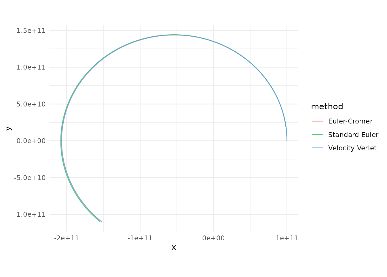

Verlet traces a clean closed ellipse, Euler-Cromer stays close but drifts slightly, and standard Euler spirals outward as it pumps energy into the orbit.

Keplerian Orbital Elements

Everything above describes how orbitr simulates — stepping positions and velocities forward using Newton’s law. But there’s an older, more elegant description of orbits that predates Newton by decades: Kepler’s laws. Johannes Kepler showed in 1609 that planetary orbits are ellipses with the Sun at one focus, and that they sweep out equal areas in equal times. These geometric properties lead to a compact way of describing any orbit with just six numbers, called the Keplerian orbital elements.

The six elements split into three groups:

Shape — how big and how stretched is the ellipse?

Semi-major axis ( $a$ ): half the longest diameter of the ellipse. Determines the orbital period through Kepler’s Third Law: $T = 2\pi\sqrt{a^3 / \mu}$ , where $\mu = GM$ is the gravitational parameter of the parent body.
Eccentricity ( $e$ ): how elongated the ellipse is. $e = 0$ is a circle; $0 < e < 1$ is an ellipse. At any point, the distance from the parent is $r = a(1-e^2)/(1 + e\cos\nu)$ .

Orientation — how is the ellipse tilted and rotated in 3D space?

Inclination ( $i$ ): the angle between the orbital plane and a reference plane (the ecliptic for solar system orbits). $0°$ is flat; $90°$ is a polar orbit.
Longitude of ascending node ( $\Omega$ ): the direction the tilt points. Measured from a reference direction to where the orbit crosses the reference plane going “upward.”
Argument of periapsis ( $\omega$ ): the angle within the orbital plane from the ascending node to the closest-approach point. Rotates the ellipse around the parent within its own plane.

Position — where is the body right now?

True anomaly ( $\nu$ ): the angle from periapsis to the body’s current position along the orbit. $0°$ is at periapsis (closest); $180°$ is at apoapsis (farthest).

From Elements to Cartesian State Vectors

orbitr’s simulation engine works entirely in Cartesian coordinates — positions $(x, y, z)$ and velocities $(v_x, v_y, v_z)$ . The function add_body_keplerian() converts Keplerian elements to Cartesian through a standard three-step procedure:

Step 1: Solve the orbit equation in the orbital plane. The distance from the parent at true anomaly $\nu$ is:

$r = \frac{a(1-e^2)}{1 + e\cos\nu}$

The position in the perifocal frame (a coordinate system where the x-axis points toward periapsis and the y-axis is 90° ahead in the direction of motion):

$x_{\text{pf}} = r\cos\nu, \quad y_{\text{pf}} = r\sin\nu$

Step 2: Compute velocity from the vis-viva relation. The specific angular momentum $h = \sqrt{\mu a(1 - e^2)}$ gives the velocity components in the perifocal frame:

$v_{x,\text{pf}} = -\frac{\mu}{h}\sin\nu, \quad v_{y,\text{pf}} = \frac{\mu}{h}(e + \cos\nu)$

These follow from conservation of angular momentum ( $h = rv_\perp$ ) and the vis-viva equation $v^2 = \mu(2/r - 1/a)$ .

Step 3: Rotate into the inertial frame. Three Euler rotations transform from the perifocal frame to the simulation’s inertial frame:

$R = R_z(-\Omega) \cdot R_x(-i) \cdot R_z(-\omega)$

This sequence first rotates by $-\omega$ to align periapsis with the ascending node, then tilts by $-i$ to incline the orbital plane, and finally rotates by $-\Omega$ to orient the node line. The resulting position and velocity are added to the parent body’s state to get absolute coordinates.

Kepler’s Laws and the Simulation

An interesting property of the Keplerian description is that it’s exact for two-body problems — a single planet orbiting a single star will follow a perfect ellipse forever. The elements are constants of motion.

In an N-body simulation like orbitr, however, the elements are only approximate because the gravitational pulls of other bodies perturb the orbit. Jupiter slightly tugs on Earth, Mars slightly tugs on Venus, and so on. Over long timescales, these perturbations cause the elements to drift — $\omega$ precesses, $e$ oscillates, inclinations wobble. This is real physics: the precession of Mercury’s perihelion was one of the first tests of General Relativity.

The Keplerian elements in add_planet() and load_solar_system() define the initial conditions at the start of the simulation. Once simulate_system() takes over, the full N-body dynamics handles all the perturbations automatically.

For a thorough walkthrough of each element with visual examples, see the Keplerian Orbital Elements vignette.

The C++ Engine

The inner acceleration loop is the computational bottleneck of any N-body simulation. orbitr ships a compiled C++ kernel (via Rcpp) that computes the $O(n^2)$ pairwise interactions in a tight nested loop. When the package is installed from source with a working C++ toolchain, simulate_system() automatically dispatches to this engine. If the compiled code isn’t available, it falls back to a vectorized R implementation that uses matrix outer products — still fast, but the C++ path is significantly faster for systems with many bodies.

You can control this with the use_cpp argument:

# Force the pure-R engine (useful for debugging or benchmarking)
simulate_system(system, use_cpp = FALSE)